[AI] 3. 신경망의 미니배치 학습 구현하기

MNIST데이터셋을 활용하여 신경망(Neural Network)의 미니배치 학습을 구현해보자.

신경망(Neural Network)은 학습을 통해 최적의 가중치(Weight)와 편향(Bias)을 찾아내야 한다. 손실 함수(Loss Function)가 최솟값일 때 가중치와 편향이 최적의 값을 갖는다.

MNIST 데이터셋

MNIST(Modified National Institute of Standards and Technology)는 머신러닝 및 딥러닝 분야에서 알고리즘의 성능을 시험하기 위해 사용하는 표준 손글씨 숫자 데이터셋이다.

총 70,000장 (학습용 60,000장, 테스트용 10,000장)으로 구성되어있다.

테스트용으로는 학습을 하지 않는다. 이는 과적합(Overfitting)이 일어나는지 확인하기 위함이다.

과적합(Overfitting)
과적합(Overfitting)은 학습 데이터에 대해 너무 과도하게 학습되어 새로운 데이터에 대한 예측 능력이 떨어지는 현상이다. 과도하게 훈련할 경우, 훈련 데이터의 노이즈나 세부적인 규칙까지 외워버리기 때문이다.

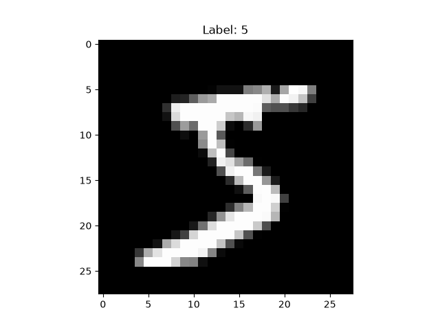
MNIST의 손글씨 데이터를 출력해보자. 출력코드와 이미지는 다음과 같다.

import numpy as np
import matplotlib.pyplot as plt
from dataset.mnist import load_mnist

# 데이터 로드
(x_train, t_train), (x_test, t_test) = load_mnist(normalize=True, one_hot_label=True)

# 확인할 이미지의 인덱스 선택
index = 0 
img = x_train[index]
label = t_train[index]

# 데이터 형태 변환 (1차원 784배열 -> 28x28 2차원 배열)
img = img.reshape(28, 28)

# 이미지 시각화
plt.imshow(img, cmap='gray')
plt.title(f"Label: {np.argmax(label)}")
plt.savefig('my_graph.png')

이미지 출력 결과는 다음과 같다.

미니배치 학습 구현

import sys, os
sys.path.append(os.path.abspath("...
sys.path.append(os.path.abspath("...

import numpy as np
import matplotlib.pyplot as plt
from dataset.mnist import load_mnist
from two_layer_net import TwoLayerNet

(x_train, t_train), (x_test, t_test) = load_mnist(normalize=True, one_hot_label=True)

train_loss_list = []

#hyperparameter
iters_num = 10000 # 반복횟수
train_size = x_train.shape[0]
batch_size = 100 #미니배치 크기
learning_rate = 0.1 #학습률

network = TwoLayerNet(input_size=784, hidden_size=50, output_size=10)

for i in range(iters_num):
  #미니배치
  batch_mask = np.random.choice(train_size, batch_size)
  x_batch = x_train[batch_mask]
  t_batch = t_train[batch_mask]

  grad = network.numerical_gradient(x_batch, t_batch)

  for key in ('W1', 'b1', 'W2', 'b2')
    network.params[key] -= learning_rate * grad[key]

  # 학습 경과
  loss = network.loss(x_batch, t_batch)
  train_loss_list.append(loss)

x = np.arange(len(train_loss_list))
plt.plot(x, train_loss_list)
plt.xlabel("iteration")
plt.ylabel("loss")
plt.xlim(0, 10000)
plt.ylim(0, 9)
plt.show()

plt.savefig('graph.png')

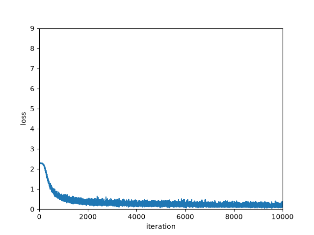
이미지 출력 결과는 다음과 같다.